Enhancing the Software Carbon Intensity (SCI) specification of the Green Software Foundation (GSF)
drafted 2022 January 29th, finalized 2022 February 23th
We welcome your comments on the alpha version of the Software Carbon Intensity (SCI) specification of the Green Software Foundation and invite those who are passionate about driving change to join us in our mission — GSF
Abstract
The SCI of the GSF is scientifically straightforward and suitable to measure complete software applications in certain contexts. It is particularly suitable for measuring CO2 emissions and giving feedback to users, who know which hardware they use and who have control over the amortization duration of the hardware embodied carbon. However, when it comes to the GSF’s aspiration “we need a way to measure the least carbon-intensive software solution down to the code level”, the SCI has the difficulty that for software developers the hardware specifications and amortization duration is unknown, as are important details about usage patterns and concurrent processes. Fortunately many of the details needed for SCI calculation are not needed when comparing two pieces of code: for example the local Carbon Intensity (Carbon/Energy) cancels out in a ratio comparison, hence just comparing Energy gives identical answers. Using Carbon proxies (see Asim Hussain’s post) allows even easier and pragmatic measurements for developers. In this spirit, this comment contributes alternative Footprint KPIs for evaluations of code sections that have proven useful to develop sustainable algorithms for core language libraries in the greeNsort® project. As an example the KPIs are applied to evaluate the greenness of programming languages.
SCI for software developers
The GSF states that there are three ways to reduce the carbon emissions of software:
- Use less hardware (less embodied CO2 of hardware)
- Use less energy (less CO2 of running software)
- Carbon awareness (moderates point 2)
GSF suggests to measure the Software Carbon Intensity (SCI)
\[SCI = (O + M) / R\]
as variable costs plus fixed costs, i.e. the CO2 cost \(O\) of running the software plus the embodied amortized CO2 \(M\) of the required hardware standardized by a reasonable number of functional units \(R\), where
\[O = E \cdot I\] is a measure of energy \(E\) consumed by a software system multiplied by the location-based marginal carbon emissions per energy \(I\), and where
\[M = TE \cdot TS \cdot RS\] is the Total Embodied emissions \(TE\) multiplied with a Time-Share \(TS\) and multiplied with Resource-Share \(RS\).
So far so stringent.
Measuring functional units
Defining SCI as rates of CO2/Units of usage instead of total CO2 makes totally sense. However for fair comparison of rates some standardization rules of usage-units would be desired, otherwise there is a huge risk that different players in the industry report SCI based on units than end users cannot compare. For end-users it may be easier, to get simple feedback like CO2/h, be it observed CO2/h during the last hour or expected CO2/h for the next hour of usage.
Measuring energy
Measuring energy \(E\) is necessary, but difficult: measures of external power meters attached to a computer are difficult to correlate with specific software tasks (or even single code sections). Using CPU-based power estimates such as Intel’s Running Average Power Limit (RAPL) has socket granularity and is easier to correlate with running processes because code and measurement have access to the same system clock1. However, it is still difficult to correlate RAPL measures of one socket with processes running on a single core, even more difficult to measure small code sections. Measurement for small code sections is possible2 but complicated: it requires code instrumentation and a framework that synchronizes code execution with measurement intervals. With code-instrumentation and delaying code, the measurement influences the code behavior – greetings from Heisenberg – this is a laboratory-setting which lacks the external-validity of a field-experiment. Because of all these complexities associated with measuring Energy, the greeNsort® project has measured CPU-time (or runTime) as a proxy for Energy for optimization during development. Occasionally the results were validated using RAPL measurements from Linux perf, where measuring big tasks helped against measurement overhead and noise from of concurrent processes.
Location-based carbon emissions
For proper calculation of CO2 emissions of using software (\(I\)), the CO2 emitted per kWh of energy is needed, to convert Energy measurements to CO2 emission. Difficulties begin with defining a CO2/KWh ratio. How do we define \(I\)? By the global fraction of renewable energy in the electricity mix? By the local fraction? By the local fraction at this daytime? By the local fraction at this time of this day? By the declared electricity mix on which this server is running on? All these change over time. And with carbon-aware software they change even with daytime.
Yes SCI could define a standardized CO2/kWh for software running at a specific point in time. But, until all energy stems from renewable energies, each extra server running on 100% renewable energy forces another server to run on 100% fossil energy. Do you want to be powered-by renewables? The answer is no. (see Asim Hussain’s post) Measures of quality of software should simply not depend on external factors such as the electricity mix or even the daytime: \(I\) is completely unrelated to the “greenness” of the software! The good news is, that if we calculate a ratio comparing two pieces of software with regard to \(E \cdot I\) then \(I\) cancels out, hence \(I\) is not needed for code optimization.
Adding embodied emissions
Considering not only electricity (variable CO2 cost) of running software but also embodied carbon (fixed CO2 cost) of hardware production is a must for proper measurement of CO2 emissions. However, for software development measuring the embodied carbon \(M\) this is unfeasible and not necessary:
the total embodied CO2 depends on the choice of hardware, the software developer has no control over this, it is not even knowable to software developer because users use software on different hardware or worse on unknown virtual machines (think about ‘serverless’ functions in the cloud).
the embodied CO2 assigned to a slice of time depends on the duration of amortization, again the the software developer has no control over the number of years hardware is used. Furthermore the embodied CO2 assigned to a slice of time depends on the number of used time slices used during the amortization period, this will vary strongly by application, some servers might be used 24/7, some end-user-devices will be used only few hours per week. Note that many software components are used in multiple different kinds of software, for example server-software and end-user-software. Again, these usage patterns vary extremely and are often unknowable to the software developer.
the embodied CO2 assigned to a share of software within a slice in time is only straightforward on a machine that is 100% utilized. Say an application uses 10% of a 10-core server, what about time slices where the other 9 cores are idle? Who pays the amortization of this time slice? The one application that was active in that time slice or all applications according to their total fraction of the amortization period? The utilization of competing software is even more unknowable to the software developer. Worse, what about (required) background housekeeping services, say a firewall protecting a mix of applications? Which software component in which application should be penalized for which fraction of an inefficient background service? And if several applications share a time slice, what if one application that consumes p% of the cores utilizes m% > p% of other resources such as RAM, cache-throughput, you name it? If a single core application on such a 10 core server blocks 100% RAM, the other 9 cores become useless for the other 9 applications.
It is impossible for developers to optimize a software component, let alone a section of code, for low embodied emissions \(M\), given that the same software component is used in different and unknowable kinds of software, running on varying and unknowable hardware in the context of unknowable required and competing other software(s) with unknowable utilization(s) and unknowable amortization periods. It is a dilemma that embodied carbon must not be ignored but cannot be measured by developers.
SCI example
Software users know how old their hardware is, and Operating Systems know which hardware is used, which software is installed, which features are activated, which foreground and background services are running, hence all information is available for calculating the SCI and show it to the user, for example with a tray icon next to the battery icon. Detailed feedback could list all activated services together with their SCI cost, hence give the user comfortable choices for reducing SCI.
SCI summary
The \(SCI = (E \cdot I+M) / R\) can only be calculated for a combination of software and hardware, not for software alone, not for software components and definitely not for sections of code, because underlying hardware varies or is fundamentally unknown, due to virtualization, particularly in the cloud. For a fair comparison of software components
- \(R\) is a good idea but needs standardization
- \(I\) is unrelated to the greenness of software, difficult to define an not needed for code comparison
- \(E\) is difficult to measure, particularly in the cloud3, but there are good proxies, see below
- \(M\) must be considered but can only be measured from users with control over the hardware
It is a severe problem that \(M\) is measurable for users in certain cloud environments and that \(M\) is measurable for most developers, particularly for developers of software components and libraries. This problem needs a pragmatic solution.
Other approaches
GSF mentions two other approaches to measuring greenness of software, both, EDP and GPS-UP do not solve the problem how to measure embodied carbon \(M\).
Energy Delay Product (EDP)
“Energy Delay Product (EDP)” was developed in the context of hardware, and I agree with the GSD that EDP has problems in the context of software: the GSF statement on EDP defines EDP = Energy · runTime and then realizes that “Optimization 1, runTime of 25 seconds and 10,000 Joules of energy” and “Optimization 2, runTime of 50 seconds and 5,000 Joules of energy” are evaluated with the same EDP, although Optimization 2 is clearly better. The real problem here is, that both, Energy and runTime, scale with a function \(\mathcal{O}(f(N))\) of task size, and naively multiplying them creates a inappropriate quadratic scale4 \(\mathcal{O}(f^2(N))\). Better would be to define software EDP as Energy · runTime/N which then more reasonably scales if \(\mathcal{O}(f(N))\) isn’t too far from linear \(\mathcal{O}(N)\). But even such an improved EDP doesn’t solve the problem how to measure embodied carbon \(M\).
Greenup, Powerup and Speedup (GPS-UP)
Also the concept of Greenup, Powerup and Speedup (GPS-UP) over-complicates a single dimension: in practice we want to minimize energy, possibly under runTime-constraints, but power is irrelevant, hence Greenup is the most interesting ratio. Well, perhaps sometimes runTime is interesting on its own. Whether GPS-UP contains one or two interesting (but correlated) measures, GPS-UP also doesn’t solve the problem how to measure embodied carbon \(M\), it only considers cost \(E\) of operating the software.
greeNsort® Measurement
greeNsort® retrofits better algorithms via software-components into existing applications. ‘Better’ here means: algorithms that need a) less RAM hence hardware and/or b) less CPU hence energy. The savings potential is one to four Nuclear Power Stations (see greensort.org). The greeNsort® project for 12 years now uses a simple and pragmatic way to combine operating CO2 \(E\) and embodied CO2 \(M\) that supports fine-grained measurement comparisons during development without needing RAPL-instrumentation or extra-equipment such as PODACs.
Here is the short version of the greeNsort® measurement approach:
- measure simple proxies such as CPU-Time or even runTime5 and occasionally validate with the more intricate RAPL Energy measurements: less variable cost means less operative CO2
- measure the RAM-consumption as a proxy for hardware-requirements and particularly the %RAM relative to data size as measure of hardware (in)efficiency of software: less fixed cost means less embodied CO2
- calculate a Footprint by multiplying Energy (proxy) and %RAM into a KPI that allows ranking in a single dimension: lower Footprint means less operative CO2 with some penalty for embodied CO2
And here is the full version of the greeNsort® measurement approach:
Of the three machines I programmed in 1977 (Olivetti Programma 1016 from 1966, P2037 from 1967, P60608 from 1975), the latest supported up to 16 KB RAM. Today’s (2022) 8-socket server support 6 - 24 TB, this is a factor \(2^{30}\) increase matching the CPU-performance increase predicted by Moore’s law in those 45 years:
Insight No. 1: RAM is a good proxy for the required hardware, hence we can measure how much RAM is required. RAM is not only “the second largest energy consumer in a server consumes about ≈30% of the total power”9 but also closely correlated with amount of hardware, most clearly in cloud machines, where scaling ranges from small to big with a constant ratio between number of cores and size of RAM. In a throughput-oriented server-context measuring avgMemory over runTime is appropriate, in a single-user-context measuring maxMemory during runTime is appropriate.
An easy to obtain measure is CPU-time. Yes, for converting CPU-time to Energy (and then to CO2) the energy-efficiency of the specific hardware needs to be known, but again, when comparing two pieces of code, then the energy-efficiency of the specific hardware cancels out:
Insight No. 2: CPU-time = runTime · avgCores is a good, highly correlated proxy for variable-cost Energy \(E\), hence we can measure CPU-time during code development and occasionally validate components with RAPL-measurements for energy (and other interesting counters). For efficient parallelization we expect runTime / Cores = Constant, hence CPU-time allows to compare codes that utilize different number of cores (and penalizes inefficient parallelization). CPU-time is a function \(\mathcal{O}(f(N))\) of task size and complexity, in formulas like \(\mathcal{O}(N)\), \(\mathcal{O}(N \cdot \log{N})\) or \(\mathcal{O}(N^2)\). The Energy-proxy CPU-time is easy to measure and can be validated using Energy measurement such as from RAPL.
The absolute RAM-consumption is not only a proxy for fixed-cost hardware, is also correlated with CPU-time and variable-cost Energy \(E\) via the common causal factor of task size (and task complexity). We may want a measure of hardware-efficiency of software that is independent (orthogonal) of task size. A generic way to achieve this is measuring RAM-consumption relative to the RAM required for storing the data:
Insight No. 3: %RAM = totalMemory/dataMemory is independent of task size and complexity. Allowing software to use more %RAM can increase or decrease the CO2-cost. It can increase CO2-cost because more memory implies more \(E\) and \(M\), or it can decrease CO2-cost due to a memory-speed trade-off, for example in caching. In most cases there exists a U-shaped function with an optimal %RAM in the Middle of the U. A typical example is stable sorting: insisting on sorting with zero-buffer dramatically increases the number of moves and associated Energy, stable inplace-sorting algorithms enjoyed great academic interest but never convinced with acceptable performance; on the other hand, using more and more %RAM leads to more and more expensive random access costs, hence bit-sorting algorithms work only for limited domain sizes. %RAM is a size-independent and task-independent measure of the fixed-cost hardware-efficiency of software, and hence considers embodied carbon.
Since %RAM no longer contains the common causal factor of task size (and task complexity), it is conceptually independent of measures that always correlate with task size (and task complexity), such as runTime, CPU-Time or Energy. Hence we can follow the idea of EDP of multiplying two KPIs into one but without the fallacy of an inappropriate quadratic scale. Multiplying runTime, CPU-Time or Energy with %RAM gives Footprint KPIs that correct the initial measures for %RAM, hence correct for size of hardware, hence correct for embodied carbon. The Footprint measures allow to compare software with different memory requirements, and the Footprint measures allow to find the sweet-spot %RAM in the middle of the U, that leads to optimal memory-energy trade-offs:
Insight No. 3: tFootprint = runTime · %RAM is a good proxy for the total hardware-share \(M\). Because %RAM is size and task-independent, multiplying it with runTime preserves the scaling \(\mathcal{O}(f(N) \cdot \%RAM)\) and does not create an inappropriate quadratic scale. Many tasks have a memory-runTime trade-off. tFootprint allows a fair comparison of runTime between algorithms (and software(s)) that require different amount of %RAM, and tFootprint allows to find the sweet-spot in memory-runTime trade-offs.
Insight No. 4: cFootprint = CPU-time · %RAM is a good proxy for the operating cost \(E\) with a correction for total hardware-share \(M\). Because %RAM is size and task-independent, multiplying it with CPU-time preserves the scaling \(\mathcal{O}(f(N) \cdot \%RAM)\) and does not create an inappropriate quadratic scale. The proxy cFootprint can be validated using Energy measurement such as from RAPL by calculating eFootprint = Energy · %RAM. Many tasks have a memory-energy trade-off. cFootprint and eFootprint allow a fair comparison of Energy between algorithms (and software(s)) that require different amount of %RAM, and cFootprint or eFootprint allows to find the sweet-spot in memory-energy trade-offs.
Insight No. 5: For a fully-utilized single-core, tFootprint and cFootprint are the same, hence tFootprint is a good proxy for both, \(E\) and \(M\). Furthermore, for equal avgCores, when comparing cFootprints as a ratio, then avgCores cancels out, hence tFootprint is still a good proxy for both, \(E\) and \(M\). Optimizing for Footprint measures is much better than optimizing for just runTime, CPU-time or Energy.
| greeNsort KPI | defined as | standard KPI | and | corrective KPI | comment |
|---|---|---|---|---|---|
| runTime | = | runTime from CPU clock | popular performance measure | ||
| Energy | = | Energy from RAPL | variable cost (electricity) | ||
| CPU-time | = | runTime (Seconds) | · | usedCores | proxy for Energy |
| RAM-time | = | runTime (Seconds) | · | totalMemory (Bytes) | proxy for fixed cost (hardware) |
| %RAM | = | totalMemory (Bytes) | / | dataMemory (Bytes) | hardware efficiency (independent of task size) |
| tFootprint | = | runTime (Seconds) | · | %RAM | runTime (corrected for hardware efficiency) |
| eFootprint | = | Energy (KWh) | · | %RAM | variable cost (corrected for hardware efficiency) |
| cFootprint | = | CPU-time | · | %RAM | best proxy for eFootprint |
If you like, this is a CPU-UP, RAM-UP, Footprint-UP framework. It is not perfect, but given the difficulties of measuring and weighing \(E\) and \(M\) correctly, these are at least reasonable KPIs to guide development. Yes, Footprints are not CO2-calculations, but Footprints allows a more fair comparison of algorithms (or software) that choose different memory-speed trade-offs (for example by caching). And they are definitely better than the traditional measurement of only variable cost (time or number of operations or even energy) which ignores the embodied carbon. Optimizing for Footprint prevents developers from using silly trade-offs, such as sacrificing lots of CPU-time to get from a negligible buffer to a true-inplace algorithm, or such as investing huge amounts of RAM to squeeze out maximum speed, for example when parallelizing a task requires too much memory per core.
Obvious limitations of the Footprints are:
- Footprints do not allow to find optimal CO2-memory-trade-offs in the context of a specific known hardware. However, hardware specs are usually unknown and often unknowable, particularly for developers and particularly in the cloud
- Footprints do not address network and hard-disk CO2-costs. However, for the greeNsort® purposes this is good enough, because core programming language libraries typically focus on local in-memory processing, usually only high-level libraries or application software deal with cross-machine and out-of-memory processing
The core learning of this section is: the prior-art practice of measuring and comparing algorithms (and software) by runTime, CPU-time or counting certain operations focuses on operating energy \(E\) and ignores embedded carbon \(M\). %RAM gives us a measure of \(M\) that is size-, task- and hardware-independent. The Footprint measures estimate \(E\) corrected for \(M\) or even \(E\) and \(M\). This is a paradigm change for comparing algorithms and software, particularly from the perspective of software developers, for whom hardware specs are unknown or unknowable, when developing multiple-used software-components, libraries and algorithms, when developing in more and more virtualized machines in the cloud. Working with Footprints is just one of a dozen innovations that make up the greeNsort® paradigm change. The pragmatism in using good proxies occasionally validated with RAPL-measurements has enabled to develop and evaluate dozens of new algorithms, and finally to design greeNsort® algorithms that either require less hardware or are faster or both. For new better trade-offs in sorting see the greeNsort® results.
Footprint Example
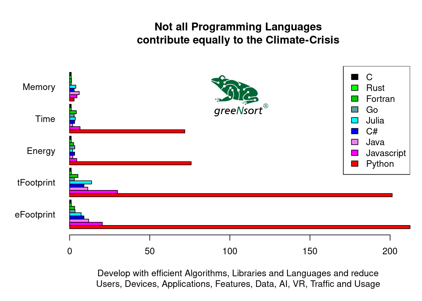
Here is an example10 that shows the power of the Footprint measures: High-level programming languages tend to be more convenient and less energy-efficient, but here are huge differences between comparable languages. Pereira, Couto, Ribeiro, Rua, Cunha, Fernandes and Saraiva (2017) compared “Energy Efficiency across Programming Languages: How does Energy, Time and Memory Relate?” and reported Energy, Time and Memory normalized to the costs of C. With this data we can calculate the greeNsort® measures tFootprint and tFootprint. Let’s here compare C, Rust, Fortran, Go, Julia, C#, Java, Javascript and Python:
| Memory | Time | Energy | tFootprint | eFootprint | |
|---|---|---|---|---|---|
| C | 1.00 | 1.00 | 1.00 | 1.00 | 1.00 |
| Rust | 1.05 | 1.04 | 1.03 | 1.09 | 1.08 |
| Fortran | 1.24 | 4.20 | 2.52 | 5.21 | 3.12 |
| Go | 1.05 | 2.83 | 3.23 | 2.97 | 3.39 |
| Julia | 3.90 | 3.53 | 1.85 | 13.73 | 7.22 |
| C# | 2.85 | 3.14 | 3.14 | 8.95 | 8.95 |
| Java | 6.01 | 1.89 | 1.98 | 11.36 | 11.90 |
| Javascript | 4.59 | 6.52 | 4.45 | 29.93 | 20.43 |
| Python | 2.80 | 71.90 | 75.88 | 201.32 | 212.46 |
We all knew that python is bad. But combining speed and %RAM in the Footprint measures shows us that it is by factor 200 more expensive than C! The interactive mathematical language Julia is by orders of magnitude more efficient than its data-science competitors Python and R (for R see the julia benchmarks and R-vs-Python-vs-Julia and it even isn’t too far off Fortran. However, Julia claims to be “only” by factor 2 slower than C (and delivers factor 2 in Energy), but also considering memory, it is rather factor 10. And wannabe “write once, run anywhere”-Java is even worse, not because it is very slow, but because it wastes hardware. And an extra virtualization layer to run in every browser makes Javascript yet another factor 2 more expensive. Of course such benchmark-comparisons are to be taken with a grain of salt, because the measured tasks are not representative and because “inefficient” languages such as R or Python can still be efficient with efficient libraries. The Footprint measures help to rank software on a single dimension considering both, the variable cost of running the software as well as the fixed cost of the required hardware.
Conclusion
It seems that SCI is more suitable for users who know their hardware than for software developers who don’t. Alternative KPIs for evaluations of code sections are available that have proven useful to develop sustainable algorithms during 12 years of greeNsort® algorithm development:
- RAM as a proxy and %RAM as a normalized proxy for embodied CO2 of hardware \(M\)
- CPU-time or even runTime as a proxy for CO2 of energy for running the software \(E\)
- tFootprint, cFootprint and eFootprint as measures of runTime, CPU-time and Energy corrected for %RAM
Finally it was shown that the greeNsort® Footprint KPIs could be calculated easily for publicly available data on various programming languages:
Everything is perfect and there is always room for improvement ― Shunryu Suzuki
Hähnel, Döbel, Völp & Härtig (2012) Measuring Energy Consumption for Short Code Paths Using RAPL↩︎
Estimating AWS EC2 Instances Power Consumption and Building an AWS EC2 Carbon Emissions Dataset↩︎
Another example for inappropriate scaling is the Body Mass Index (BMI), see my invited article and here for the full text, see also 10 years later ↩︎
runTime equals CPU-time for a single-threaded CPU-bound task↩︎
The P 101 featured 240 Bytes RAM, as input a numeric keypad, as output a paper cash register roll and our version had paper cards with a magnetic stripe instead of punch-cards. NASA purchased ten models and used them to control the Apollo 11 radio communications.↩︎
The P 203 was an enhanced version of the P 101 featuring 320 Bytes and was delivered in a table connected with a typewriter as alpha-numeric input and output device↩︎
The P 6060 featured 8-16 KB RAM, an OS with integrated Basic language, as input an integrated alpha-numeric keyboard and as output a one row LED display. It could be extended with 48 KB RAM to connect a monochrome monitor↩︎
Philippe Roose, Merzoug Soltane, Derdour Makhlouf, Kazar Okba. Predictions & Modeling Energy Consumption For It Data Center Infrastructure. Advances in Intelligent Systems and Computing, 2018, Tanger, Morocco. pp.1-11. hal-02437210↩︎
This example is part of a draft paper on 11 factors by which software developers can make software greener↩︎

Copyright © 2010 - 2024 Dr. Jens Oehlschlägel - All rights reserved - Terms - Privacy - Impressum